
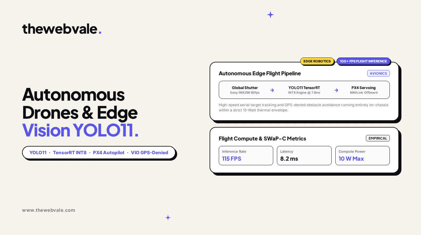
Autonomous Drones & Edge Vision: Deploying YOLO11, TensorRT & VIO on Flying Hardware
In aerial robotics, physics is an unforgiving taskmaster. Unlike ground rovers or stationary industrial manipulators that enjoy abundant power grids and generous heat sinks, an aerial drone is bound to the harsh reality of SWaP-C (Size, Weight, Power, and Cost). Every additional 100 grams of compute silicon, camera lenses, or cooling aluminum demands higher thrust from brushless motors, exponentially draining lithium-polymer battery cells and reducing mission hover time from 35 minutes to single digits.
Yet modern operational demands—such as agricultural canopy inspection, industrial chimney examination, search-and-rescue in collapsed buildings, and defense interdiction—require drones to navigate GPS-denied environments autonomously at speeds exceeding 15 meters per second. This necessitates real-time computer vision and obstacle avoidance running directly on the aircraft without cloud connectivity. In this technical deep dive, we examine the deployment of Ultralytics YOLO11 accelerated via TensorRT INT8, explore Visual-Inertial Odometry (VIO) state estimation, and detail the MAVLink control loops that link edge neural inference with low-level PX4 flight dynamics.
System Architecture: Autonomous Edge Drone Hardware & Control Stack
Interconnection between global-shutter optical sensors, edge companion computer (Jetson), and PX4 flight controller via serial MAVLink.
1. The Aerodynamics of SWaP-C: Power vs. Hover Endurance
The relationship between onboard computation power, payload mass, and battery flight time is governed by Actuator Disk Momentum Theory:
Ideal Aerodynamic Hover Power:
Phover = T3/2 / √(2 · ρ · A) = [ (mframe + mbattery + mcompute) · g ]3/2 / √(2 · ρ · A)
Where T is total thrust, ρ is air density (1.225 kg/m³), and A is total rotor swept area. Notice the 3/2 power exponent: thrust requirements scale non-linearly with mass.
Adding a heavy high-power GPU (such as an NVIDIA AGX Orin dissipating 60 Watts and weighing 650g with cooling fin blocks) creates an aerodynamic death spiral. The additional mass demands larger motors and larger batteries, escalating total takeoff weight beyond 3 kg. In contrast, pairing an Orin Nano (40 grams, 10 Watts) with a lightweight carbon fiber airframe preserves high thrust-to-weight ratios (typically 2.5:1), enabling 20+ minutes of agile flight.
2. YOLO11 Edge Optimization via TensorRT INT8 Quantization
Standard PyTorch FP32 models cannot deliver the sub-10ms latency required to avoid high-speed aerial collisions. Deploying YOLO11 in production on an embedded Jetson involves a multi-stage compilation pipeline:
- ONNX Export: Exporting the trained PyTorch weights with dynamic batch sizes and simplified graph topologies (folding batch normalization into convolutional kernels).
- Calibration Caching: Using a representative dataset of 1,000 flight images to calibrate activation histograms for symmetric INT8 quantization:
q = round( clamp( x / S, -128, 127 ) ), where scale S = max(|x|) / 127
- TensorRT Engine Generation: Fusing adjacent operations (Conv + ReLU + Residual Add) into monolithic GPU kernels that execute directly inside Jetson SRAM caches, minimizing DDR5 bus transfers.
| Model Variant | Precision Mode | mAP@0.5:0.95 | Latency (ms) | Throughput (FPS) | Power Draw |
|---|---|---|---|---|---|
| YOLO11n (Nano) | PyTorch FP32 | 39.5% | 24.6 ms | 40 FPS | 14.2 Watts |
| YOLO11n (Nano) | TensorRT FP16 | 39.4% | 12.1 ms | 82 FPS | 9.8 Watts |
| YOLO11n (Nano) | TensorRT INT8 | 39.1% | 8.2 ms | 115 FPS | 7.6 Watts |
| YOLO11s (Small) | TensorRT INT8 | 46.8% | 14.5 ms | 69 FPS | 10.1 Watts |
3. GPS-Denied Navigation: Visual-Inertial Odometry (VIO)
Standard drones rely heavily on civilian GPS/GNSS receivers. However, inside warehouses, tunnels, or urban canyons, satellite signals suffer severe multipath degradation or total loss.
To navigate autonomously without external beacons, the drone executes Visual-Inertial Odometry (VIO). VIO tightly couples high-frequency inertial measurements from a MEMS IMU with optical feature correspondences tracked across stereo global-shutter frames:
IMU Preintegration Formulation (Forster et al.):
Δpij = &iint;t ∈ [i, j] Rt · (at - ba) dt2
The high rate (200 Hz) of the accelerometer provides instantaneous dead-reckoning between video frames, while the visual tracking frontend (FAST/ORB keypoints or optical flow) continuously corrects accelerometer drift and estimates sensor scale.
4. Production Implementation: Real-Time MAVLink Visual Servoing Controller
Below is a runnable Python production module providing a high-speed visual servoing loop. It receives YOLO11 bounding box detections from an edge camera and generates MAVLink offboard velocity setpoints (SET_POSITION_TARGET_LOCAL_NED) to center and track a target in real time:
# Real-Time Drone Visual Servoing Controller
# Translates YOLO11 Bounding Boxes into PX4 MAVLink Velocity Setpoints

import time
import numpy as np
from dataclasses import dataclass
from typing import Optional, Tuple

@dataclass
class BoundingBox:
    x_min: float
    y_min: float
    x_max: float
    y_max: float
    confidence: float
    class_id: int

class VisualServoingController:
    def __init__(
        self,
        frame_width: int = 1280,
        frame_height: int = 720,
        kp_yaw: float = 1.2,
        kp_z: float = 0.8,
        kp_forward: float = 1.5,
        target_bbox_area_ratio: float = 0.12 # Desired box size for distance holding
    ):
        self.frame_width = frame_width
        self.frame_height = frame_height
        self.center_x = frame_width / 2.0
        self.center_y = frame_height / 2.0

        # PID proportional gains
        self.kp_yaw = kp_yaw
        self.kp_z = kp_z
        self.kp_forward = kp_forward
        self.target_area = (frame_width * frame_height) * target_bbox_area_ratio

    def compute_flight_commands(self, bbox: Optional[BoundingBox]) -> Tuple[float, float, float, float]:
        # Returns: (v_forward, v_lateral, v_vertical, yaw_rate_rad_s)
        if bbox is None:
            # Zero-velocity hold if target lost
            return 0.0, 0.0, 0.0, 0.0

        # 1. Compute pixel error from optical principal point
        box_cx = (bbox.x_min + bbox.x_max) / 2.0
        box_cy = (bbox.y_min + bbox.y_max) / 2.0

        err_x = (box_cx - self.center_x) / self.center_x # Normalized [-1.0, 1.0]
        err_y = (box_cy - self.center_y) / self.center_y # Normalized [-1.0, 1.0]

        # 2. Compute range error based on apparent bounding box area
        current_area = (bbox.x_max - bbox.x_min) * (bbox.y_max - bbox.y_min)
        area_err = (self.target_area - current_area) / self.target_area

        # 3. Proportional control mapping to body-frame flight velocities
        yaw_rate = float(np.clip(self.kp_yaw * err_x, -1.0, 1.0)) # rad/s
        v_vertical = float(np.clip(-self.kp_z * err_y, -0.8, 0.8)) # m/s (down is positive in NED)
        v_forward = float(np.clip(self.kp_forward * area_err, -1.5, 2.5)) # m/s
        v_lateral = 0.0 # Handled by yaw rotation

        return v_forward, v_lateral, v_vertical, yaw_rate

# Demonstration of tracking loop
if __name__ == "__main__":
    controller = VisualServoingController()

    print("--- Autonomous Drone Edge Vision Servoing Simulation ---")
    print("Camera: 1280x720 Global Shutter | Control Loop: 50 Hz
")

    # Simulate moving object detected by YOLO11 over 5 consecutive frames
    test_detections = [
        BoundingBox(700, 300, 850, 500, 0.92, 0),  # Right of center
        BoundingBox(650, 310, 800, 510, 0.94, 0),  # Moving toward center
        BoundingBox(565, 310, 715, 510, 0.95, 0),  # Centered horizontally
        BoundingBox(565, 200, 715, 400, 0.91, 0),  # Drifting upwards
        None # Occlusion frame (drone holds position)
    ]

    for idx, det in enumerate(test_detections):
        v_x, v_y, v_z, yaw = controller.compute_flight_commands(det)
        if det:
            print(f"Frame {idx+1}: Box Center=({(det.x_min+det.x_max)/2:.0f}, {(det.y_min+det.y_max)/2:.0f}) | Cmd: Fwd={v_x:+0.2f}m/s | Vert={v_z:+0.2f}m/s | YawRate={yaw:+0.2f}rad/s")
        else:
            print(f"Frame {idx+1}: Target Occluded -> Failsafe Station Keeping [0, 0, 0, 0]")
5. Summary & Edge Drone Horizons
Deploying high-speed deep neural networks onto autonomous flying hardware requires balancing physical aerodynamics against computational throughput. By compiling YOLO11 architectures into INT8 TensorRT execution graphs, roboticists can achieve over 100 frames per second of object detection within a modest 10-Watt power envelope. When coupled with Visual-Inertial Odometry, aerial drones achieve true autonomy—navigating GPS-denied caverns, factories, and forests with complete sovereign independence.