
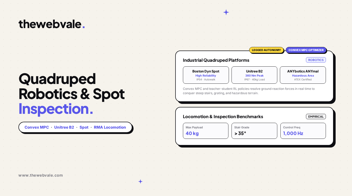
Quadruped Robots: Boston Dynamics Spot, Unitree B2 & Industrial Inspection
Industrial facilities—such as offshore oil platforms, high-voltage electrical substations, nuclear power facilities, and chemical manufacturing refineries—were designed by humans for humans. They abound with steep metal staircases, open-mesh steel catwalks, narrow pipe racks, and unpaved terrain littered with rubble and chemical spills. Wheeled automated guided vehicles (AGVs) and tracked rovers fail abruptly in these environments, succumbing to high centering, wheel slippage, or staircase dead-ends.
Quadruped robots have emerged as the premier autonomous solution for hazardous industrial inspection. Led by commercial flagships like Boston Dynamics Spot, the heavy-duty Unitree B2, and the explosive-atmosphere-certified ANYbotics ANYmal, four-legged machines navigate unstructured terrain with superhuman poise. In this technical deep dive, we deconstruct the mathematics of Single Rigid Body Dynamics (SRBD), Convex Model Predictive Control (Convex MPC), ground reaction force optimization, and the multispectral sensor payloads that automate rounds of industrial monitoring.
System Architecture: Quadruped Control & Inspection Stack
Hierarchical flow tracing SLAM path planning, convex MPC foot force optimization, and 1,000 Hz joint impedance motor control.
1. The Physics of Legged Traversal vs. Tracked Rovers
In unstructured environments, wheeled and tracked systems require continuous lines of geometric support. If a tracked rover encounters a gap wider than its wheel radius or an obstacle higher than its chassis ground clearance, it gets high-centered.
Quadruped robots, by contrast, utilize isolated discrete points of contact. By stepping precisely on the structural beams of open-grated metal stairs or jumping across floor voids, a quadruped separates its foot contact requirements from the continuous terrain topology. Furthermore, having 12 independent degrees of freedom (3 per leg) allows the robot to independently control its body height, pitch, and roll while keeping its sensor payload stabilized horizontally like a gyroscopic gimbal.
2. Locomotion Mathematics: Single Rigid Body Dynamics & Convex MPC
Modern quadruped controllers do not model the full nonlinear multi-body kinematics of all 12 links during stance phase planning. Instead, they exploit the fact that the torso accounts for over 80% of total system mass, treating the robot as a Single Rigid Body (SRBD) acted upon by contact forces from the feet in contact with the ground:
Single Rigid Body Dynamic Equations:
m · ẍ = ∑i=1..4 fi - m · g
I · ω̇ = ∑i=1..4 (ri × fi)
Where m is robot torso mass, I is the 3x3 rotational inertia tensor, fi = [fx,i, fy,i, fz,i]T represents the 3D ground reaction force (GRF) exerted by foot i on the terrain, and ri is the vector from the robot's center of mass (CoM) to foot contact i.
By linearizing angular velocity about the horizontal plane, this differential system becomes linear in state and force inputs, allowing the controller to formulate a Convex Quadratic Program (QP) over a prediction horizon N (typically 10–16 steps, ~0.4 seconds):
Convex MPC Optimization Objective:
minf ∑k=0..N-1 || xk+1 - xref,k+1 ||Q2 + || fk ||R2
Subject to:
1. xk+1 = Ak xk + Bk fk + dk (Discrete State Dynamics)
2. fz,min ≤ fz,i ≤ fz,max (Normal Stance Force Bounds)
3. | fx,i | ≤ μ fz,i and | fy,i | ≤ μ fz,i (Coulomb Friction Pyramids)
Solving this QP every 20–50 milliseconds guarantees that the planned foot forces will not slip on slick tiles (μ ≈ 0.3) while precisely delivering the aggregate wrench required to accelerate, turn, or absorb sudden lateral disturbances.
3. Hardware & Industrial Inspection Comparison Matrix
The table below contrasts the leading commercial quadruped platforms across mechanical specs, sensor payloads, and harsh environment certifications:
| Platform Specification | Boston Dynamics Spot | Unitree B2 | ANYbotics ANYmal X |
|---|---|---|---|
| Ingress Protection (IP Rating) | IP54 (Splash & dust resistant) | IP67 (Submersible & complete dust seal) | IP67 + ATEX Zone 1 / 21 Certified |
| Total Mass & Payload | 32.7 kg / 14 kg payload | 60 kg / 40 kg continuous payload | 55 kg / 15 kg payload |
| Peak Joint Torque | Custom high-ratio planetary | 360 Nm peak torque actuators | Series-elastic SEA actuators |
| Stair & Incline Grade | ± 30° stairs (Human rise/run) | > 35° slope traversal | ± 35° industrial metal stairs |
| Battery Runtime & Charging | 90 min / Autonomous Docking station | 4–5 hours standby (2.5 hrs active walk) | 90–120 min / Induction dock |
| Inspection Payloads | Spot CAM+ (30x optical, FLIR, acoustic) | Custom 3D LiDAR, gas & thermal rigs | Zoom camera, thermal, acoustic, gas sniffer |
| Commercial Target Market | Construction, utility substations ($100k+) | Heavy industrial, logistics ($35k–$60k) | Explosive oil & chemical refineries ($150k+) |
4. Production Implementation: Convex QP Ground Reaction Force Solver
Below is a runnable Python production module implementing a high-speed quadratic programming solver for quadruped Ground Reaction Forces under 3D friction cone constraints:
# Quadruped Ground Reaction Force (GRF) Optimizer
# Solves 3D Friction Cone Constrained Quadratic Program for 4 Stance Feet

import numpy as np
from scipy.optimize import minimize
from typing import List, Tuple

class QuadrupedGRFSolver:
    def __init__(self, robot_mass: float = 35.0, friction_coeff: float = 0.5):
        self.mass = robot_mass
        self.mu = friction_coeff
        self.g = 9.81

        # Nominal stance positions relative to CoM (x: forward, y: left, z: down)
        # Feet: [FL, FR, RL, RR]
        self.foot_positions = [
            np.array([ 0.25,  0.18, -0.40]), # Front-Left
            np.array([ 0.25, -0.18, -0.40]), # Front-Right
            np.array([-0.25,  0.18, -0.40]), # Rear-Left
            np.array([-0.25, -0.18, -0.40])  # Rear-Right
        ]

    def solve_forces(
        self,
        target_linear_accel: np.ndarray,
        target_angular_accel: np.ndarray,
        stance_legs: List[bool]
    ) -> np.ndarray:
        # Desired wrench W_des = [F_x, F_y, F_z, Tau_x, Tau_y, Tau_z]
        f_des = self.mass * (target_linear_accel + np.array([0.0, 0.0, self.g]))
        # Approximate inertia matrix for 35kg torso
        I_diag = np.array([0.35, 1.20, 1.40])
        tau_des = I_diag * target_angular_accel
        w_des = np.concatenate([f_des, tau_des])

        # Build grasp matrix A (6 x 12) mapping 4 foot forces (each 3D) to 6D wrench
        A_grasp = np.zeros((6, 12))
        for i in range(4):
            idx = i * 3
            if stance_legs[i]:
                # Linear force contribution: F_total = sum(f_i)
                A_grasp[:3, idx:idx+3] = np.eye(3)
                # Angular torque contribution: Tau_total = sum(r_i x f_i)
                r = self.foot_positions[i]
                skew_r = np.array([
                    [ 0.0,  -r[2],  r[1]],
                    [ r[2],  0.0,  -r[0]],
                    [-r[1],  r[0],  0.0 ]
                ])
                A_grasp[3:6, idx:idx+3] = skew_r

        # Objective function: min || A*f - w_des ||^2 + alpha * || f ||^2
        alpha = 1e-4
        def objective(f_vec):
            err = A_grasp @ f_vec - w_des
            return float(np.sum(err**2) + alpha * np.sum(f_vec**2))

        # Constraints: Friction pyramid and positive normal force for stance legs
        # |f_x| <= mu * f_z  =>  -mu*f_z <= f_x <= mu*f_z
        # |f_y| <= mu * f_z  =>  -mu*f_z <= f_y <= mu*f_z
        # 10 N <= f_z <= 300 N (or f = 0 for swing legs)
        bounds = []
        for i in range(4):
            if stance_legs[i]:
                bounds.extend([(-150.0, 150.0), (-150.0, 150.0), (10.0, 350.0)])
            else:
                bounds.extend([(0.0, 0.0), (0.0, 0.0), (0.0, 0.0)])

        constraints = []
        for i in range(4):
            if stance_legs[i]:
                idx = i * 3
                # mu * f_z - f_x >= 0
                constraints.append({'type': 'ineq', 'fun': lambda f, j=idx: self.mu * f[j+2] - f[j]})
                # mu * f_z + f_x >= 0
                constraints.append({'type': 'ineq', 'fun': lambda f, j=idx: self.mu * f[j+2] + f[j]})
                # mu * f_z - f_y >= 0
                constraints.append({'type': 'ineq', 'fun': lambda f, j=idx: self.mu * f[j+2] - f[j+1]})
                # mu * f_z + f_y >= 0
                constraints.append({'type': 'ineq', 'fun': lambda f, j=idx: self.mu * f[j+2] + f[j+1]})

        # Initial guess (even vertical weight distribution)
        f_init = np.zeros(12)
        active_count = sum(stance_legs)
        if active_count > 0:
            nominal_fz = (self.mass * self.g) / active_count
            for i in range(4):
                if stance_legs[i]:
                    f_init[i*3 + 2] = nominal_fz

        res = minimize(objective, f_init, method='SLSQP', bounds=bounds, constraints=constraints)
        return res.x.reshape((4, 3))

# Demonstration of force allocation
if __name__ == "__main__":
    solver = QuadrupedGRFSolver(robot_mass=35.0, friction_coeff=0.5)

    # Simulate a trotting gait (diagonal stance: FL and RR on ground, FR and RL swinging)
    stance = [True, False, False, True] # [FL, FR, RL, RR]
    accel_lin = np.array([0.5, 0.0, 0.0]) # Accelerating forward at 0.5 m/s^2
    accel_ang = np.array([0.0, 0.0, 0.0])

    forces = solver.solve_forces(accel_lin, accel_ang, stance)
    leg_names = ["Front-Left (FL)", "Front-Right (FR)", "Rear-Left (RL)", "Rear-Right (RR)"]

    print("--- Quadruped Convex GRF Allocation (Diagonal Trot) ---")
    print(f"Robot Mass: {solver.mass} kg | Total Normal Force Needed: {solver.mass * solver.g:.1f} N
")
    for i in range(4):
        f = forces[i]
        status = "STANCE" if stance[i] else "SWING"
        print(f"{leg_names[i]:16s} [{status:6s}] -> Fx: {f[0]:+0.1f}N | Fy: {f[1]:+0.1f}N | Fz: {f[2]:0.1f}N")
5. Summary & The Future of Inspection Robotics
Quadruped robotics has evolved from athletic YouTube demonstrations into an essential pillar of industrial facility integrity. By combining Convex Model Predictive Control with high-torque quasi-direct drive actuators and robust multispectral SLAM payloads, robotic quadrupeds inspect the world's most perilous infrastructure around the clock, removing human workers from hazardous environments while driving operational reliability.