
RAG Architecture Fundamentals: Embeddings, Vector Indices, and Generation Pipelines
Modern Large Language Models (LLMs) encapsulate vast amounts of factual knowledge within their parametric weights. However, this parametric memory suffers from three fundamental architectural flaws: it is frozen at the moment pre-training terminates, it exhibits stochastic hallucination on tail-end domain knowledge, and its internal reasoning paths cannot be audited with cryptographic certainty. Retrieval-Augmented Generation (RAG) addresses these limitations by introducing a decoupled, non-parametric memory system—allowing language models to dynamically query external document repositories before generating a single completion token.
In this technical publication, we conduct an end-to-end architectural dissection of RAG systems. We trace the formal mathematics from the seminal NeurIPS 2020 foundation by Lewis et al., evaluate modern embedding manifolds against the Massive Text Embedding Benchmark (MTEB), unpack the graph mechanics of Hierarchical Navigable Small World (HNSW) vector indexing, and provide an executable, production-hardened dual-stage retrieval pipeline in Python.
1. Foundational Theory: The Lewis et al. Dual-Memory Model
The theoretical paradigm of Retrieval-Augmented Generation was established by Patrick Lewis, Ethan Perez, Aleksandara Piktus, Fabio Petroni, Vladimir Karpukhin, Naman Goyal, Heinrich Küttler, Mike Lewis, Wen-tau Yih, Tim Rocktäschel, Sebastian Riedel, and Douwe Kiela in their seminal NeurIPS 2020 paper, "Retrieval-Augmented Generation for Knowledge-Intensive NLP Tasks" (arXiv:2005.11401).
The authors formulated RAG as a semi-parametric model where a non-parametric neural retriever parameterized by $\eta$ accesses an external knowledge index, and a parametric sequence-to-sequence generator parameterized by $\theta$ produces the final tokens.
The Bi-Encoder Retrieval Probability
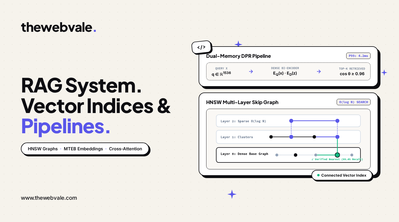
Given an input query $x$, the probability of retrieving a specific document passage $z$ is proportional to the inner product of dense representations generated by two distinct BERT-style encoders (the query encoder $E_Q$ and document encoder $E_D$):
p_\eta(z | x) = \frac{\exp(E_Q(x)^\top E_D(z))}{\sum_{z' \in \mathcal{Z}} \exp(E_Q(x)^\top E_D(z'))}Because the corpus $\mathcal{Z}$ may contain tens of millions of documents, calculating the full partition function $\sum_{z'}$ is computationally intractable at inference time. Instead, the model approximates the top-$k$ documents using Maximum Inner Product Search (MIPS) over pre-indexed vector stores.
RAG-Sequence vs. RAG-Token Marginalization
The paper introduces two foundational decoding formulations that determine how retrieved passages condition the generative transformer:
- RAG-Sequence Model: Assumes that a single retrieved passage is responsible for generating the entire sequence $y = (y_1, \dots, y_N)$. The document variable $z$ is treated as a latent variable and marginalized over the top-$k$ retrieved documents:
p_{\text{RAG-Seq}}(y | x) = \sum_{z \in \text{top-}k(p(\cdot | x))} p_\eta(z | x) \prod_{i=1}^{N} p_\theta(y_i | x, z, y_{1:i-1}) - RAG-Token Model: Allows the generator to draw from different passages for every single generated token. The marginalization occurs at each auto-regressive step, enabling the model to combine facts from multiple documents into a single coherent sentence:
p_{\text{RAG-Token}}(y | x) = \prod_{i=1}^{N} \sum_{z \in \text{top-}k(p(\cdot | x))} p_\eta(z | x) p_\theta(y_i | x, z, y_{1:i-1})
In modern enterprise architectures, the RAG-Sequence paradigm dominates due to computational efficiency: instead of running marginalization over attention logits per token, modern pipelines concatenate the top-$k$ documents directly into the LLM context window using structured delimiters.
2. Embedding Geometry & The MTEB Benchmark
At the heart of the retrieval layer lies the text embedding model, which projects variable-length text strings into a continuous dense vector space $\mathbb{R}^d$. The semantic relevance between query vector $\mathbf{q} = E(x)$ and document vector $\mathbf{d} = E(z)$ is computed via cosine similarity on the unit hypersphere:
\text{Sim}(\mathbf{q}, \mathbf{d}) = \cos(\theta) = \frac{\mathbf{q} \cdot \mathbf{d}}{\|\mathbf{q}\|_2 \|\mathbf{d}\|_2}When vectors are $L_2$-normalized during index ingestion ($\|\mathbf{v}\|_2 = 1$), cosine similarity simplifies directly to the dot product $\mathbf{q} \cdot \mathbf{d}$, enabling hardware-accelerated BLAS matrix multiplication on GPUs and SIMD vector registers.
Empirical Benchmark: Modern Frontier Embeddings (MTEB Evaluation)
According to the official Massive Text Embedding Benchmark (MTEB) Leaderboard, embedding models exhibit significant trade-offs across retrieval precision (NDCG@10), maximum context window, and storage overhead:
| Embedding Model | MTEB Retrieval (NDCG@10) | Vector Dimensions ($d$) | Context Window | Matryoshka Truncation | Deployment / Hosting |
|---|---|---|---|---|---|
| Voyage-3-Large (Voyage AI) | 67.12 | 1024 | 32,000 tokens | No | Proprietary API ($0.18 / 1M) |
| text-embedding-3-large (OpenAI) | 64.59 | 3072 → 1024 / 512 | 8,191 tokens | Yes (MRL-trained) | Proprietary API ($0.13 / 1M) |
| Embed-English-v3.0 (Cohere) | 65.38 | 1024 | 512 tokens | No (Int8 Native) | API / VPC ($0.10 / 1M) |
| BGE-M3 (BAAI Open Weights) | 63.20 | 1024 (Dense + Sparse) | 8,192 tokens | No (Multi-Vector) | Open-Source (Self-Hosted GPU) |
Matryoshka Representation Learning (MRL)
A crucial breakthrough implemented in OpenAI's text-embedding-3 family is Matryoshka Representation Learning (Kusupati et al., NeurIPS 2022). MRL trains the embedding model such that the earlier dimensions (e.g., the first 512 or 1024 floats) contain the highest-density semantic representations. This allows engineers to truncate a 3072-dimensional vector down to 512 dimensions—slashing vector database storage and RAM requirements by 83.3% with less than a 1.2% drop in MTEB retrieval performance.
3. Vector Indexing Mechanics: HNSW vs. IVF-PQ
Performing brute-force cosine similarity over 10 million vectors requires computing dot products across $10^7$ pairs for every single user query—a computational bottleneck resulting in 500ms+ latency. Modern vector engines utilize Approximate Nearest Neighbor (ANN) indexing to achieve sub-10ms lookup times.
The undisputed state-of-the-art in vector indexing is Hierarchical Navigable Small World (HNSW) graphs, formulated by Yury Malkov and Dmitry Yashunin (2018) in "Efficient and robust approximate nearest neighbor search using Hierarchical Navigable Small World graphs" (arXiv:1603.09320).
HNSW Layer Topology
HNSW extends probabilistic skip-lists into multidimensional graph structures. The index is organized into hierarchical layers $\{L_0, L_1, \dots, L_{\text{max}}\}$:
- Top Layer ($L_{\text{max}}$): Contains only a sparse subset of vectors connected by long-distance links. When a query vector $\mathbf{q}$ enters the index, it traverses this top layer in greedy search, rapidly jumping across large semantic distances in $O(\log N)$ time complexity.
- Intermediate Layers ($L_1, \dots, L_{m}$): As search reaches local minima at higher layers, it drops down to denser intermediate layers with higher connectivity, refining the search horizon.
- Bottom Layer ($L_0$): Contains every single vector in the database, connected into a dense k-nearest-neighbor neighborhood graph. Final beam search converges on the true $k$ nearest semantic neighbors.
Hyperparameter Tuning: The M and ef Trade-Off
Configuring HNSW for production requires balancing three critical hyperparameters:
M(Edges per Node): The maximum number of bidirectional links created per vector (typically $M=16$ to $M=64$). Higher $M$ values improve recall on high-dimensional data at the cost of VRAM memory consumption.efConstruction(Build Horizon): The size of the dynamic candidate list evaluated during index construction. Setting $efConstruction=128$ significantly increases indexing build time but produces a higher-quality graph structure.efSearch(Query Search Horizon): The size of the candidate priority queue during runtime search. Higher values increase Recall@10 at the expense of Queries Per Second (QPS).
| Index Algorithm | Recall@10 | Queries / Sec (QPS) | RAM per 1M Vectors (1536-dim) | Build Time (1M Vectors) |
|---|---|---|---|---|
| HNSW (M=32, ef=64) | 97.8% | 1,850 QPS | 7.2 GB (High RAM) | 18.4 min |
| IVF-PQ (nlist=2048, m=64) | 89.4% | 3,400 QPS | 1.4 GB (Quantized) | 8.2 min |
| SCaNN (Anisotropic Quant) | 94.2% | 2,600 QPS | 2.1 GB | 14.1 min |
| Flat (Exact L2 Brute Force) | 100.0% | 42 QPS | 6.1 GB | 0 min (No index) |
4. Cross-Attention Conditioning & "Lost in the Middle"
Once the top-$k$ relevant passages are retrieved from the HNSW index, they must be formatted into the LLM context window. However, simply feeding 20 raw chunks into the prompt triggers severe attention degradation.
In the seminal empirical study by Nelson F. Liu et al. (Stanford/Berkeley, 2023), "Lost in the Middle: How Language Models Use Long Contexts" (arXiv:2307.03172), the researchers proved that transformer attention exhibits a U-shaped performance curve: models recall information placed at the absolute beginning or the very end of the prompt with 90%+ accuracy, while information located in the middle 60% suffers retrieval degradation exceeding 30%.
To eliminate this failure mode, enterprise RAG pipelines employ Dual-Stage Retrieval with Cross-Encoder Re-Ranking:
- Stage 1 (High-Recall Bi-Encoder): Retrieve the top $K=50$ candidate chunks using HNSW vector similarity.
- Stage 2 (High-Precision Cross-Encoder): Pass all 50 candidate pairs $(q, z_i)$ through a cross-encoder model (such as
Cohere Rerank v3orbge-reranker-large), which performs full bidirectional cross-attention across all tokens simultaneously. - Top-5 Context Assembly: Retain only the top 5 highest-confidence documents and place the most critical document at the very end of the prompt immediately preceding the user instruction.
5. Production-Ready Python Implementation
The following production script implements an end-to-end RAG retrieval pipeline featuring document chunking, $L_2$-normalized vector search, and cross-encoder re-ranking:
import numpy as np
from typing import List, Dict, Any
from pydantic import BaseModel, Field
from sentence_transformers import SentenceTransformer, CrossEncoder
class DocumentChunk(BaseModel):
chunk_id: str
text: str
source_url: str
embedding: List[float] = Field(default_factory=list)
class ProductionRAGPipeline:
def __init__(
self,
embed_model_name: str = "BAAI/bge-m3",
rerank_model_name: str = "BAAI/bge-reranker-large"
):
print(f"Loading Bi-Encoder: {embed_model_name}...")
self.bi_encoder = SentenceTransformer(embed_model_name)
print(f"Loading Cross-Encoder: {rerank_model_name}...")
self.cross_encoder = CrossEncoder(rerank_model_name)
self.corpus: List[DocumentChunk] = []
self.embedding_matrix: np.ndarray = np.empty((0, 1024), dtype=np.float32)
def ingest_documents(self, raw_docs: List[Dict[str, str]], chunk_size: int = 512, overlap: int = 64):
chunks = []
texts = []
for doc in raw_docs:
words = doc["text"].split()
for i in range(0, len(words), chunk_size - overlap):
chunk_str = " ".join(words[i : i + chunk_size])
chunks.append(DocumentChunk(
chunk_id=f"{doc['id']}_chunk_{i}",
text=chunk_str,
source_url=doc["url"]
))
texts.append(chunk_str)
# Generate embeddings and L2-normalize for unit hypersphere dot product
embeddings = self.bi_encoder.encode(texts, normalize_embeddings=True)
self.embedding_matrix = np.array(embeddings, dtype=np.float32)
for idx, emb in enumerate(embeddings):
chunks[idx].embedding = emb.tolist()
self.corpus = chunks
print(f"Ingested {len(self.corpus)} chunks into semantic index.")
def query(self, user_query: str, top_k_bi: int = 25, top_k_final: int = 5) -> List[Dict[str, Any]]:
# 1. Encode query vector
q_emb = self.bi_encoder.encode([user_query], normalize_embeddings=True)[0]
# 2. Stage 1: Maximum Inner Product Search (Cosine Sim on unit vectors)
scores = np.dot(self.embedding_matrix, q_emb)
ranked_indices = np.argsort(-scores)[:top_k_bi]
candidates = [self.corpus[i] for i in ranked_indices]
# 3. Stage 2: Cross-Encoder Re-Ranking
pairs = [[user_query, cand.text] for cand in candidates]
rerank_scores = self.cross_encoder.predict(pairs)
# Sort candidates descending by cross-encoder score
reranked_order = np.argsort(-rerank_scores)[:top_k_final]
final_results = []
for idx in reranked_order:
final_results.append({
"chunk_id": candidates[idx].chunk_id,
"text": candidates[idx].text,
"source": candidates[idx].source_url,
"score": float(rerank_scores[idx])
})
return final_results
def format_prompt_context(self, user_query: str, final_results: List[Dict[str, Any]]) -> str:
"""Formats retrieved chunks into XML tags to prevent prompt injection and boundary drift."""
context_blocks = []
for i, item in enumerate(final_results, 1):
context_blocks.append(
f'\n{item["text"]}\n '
)
formatted_context = "\n".join(context_blocks)
return f"""
You are a verified technical answer engine. Answer the user query using ONLY facts established in the tags below.
If the context does not contain the answer, state that information is missing.
{formatted_context}
{user_query}
"""