
Tactile Sensing in Robotics: Artificial Skin, Optical Elastomers & Touch Manipulation
Try closing your eyes and picking a single credit card out of a leather wallet, or holding a ripe raspberry without crushing its delicate cell walls. A human accomplishes these tasks effortlessly through cutaneous mechanoreceptors: over 17,000 tactile sensory units embedded in the human hand that continuously stream high-bandwidth signals of contact geometry, skin stretch, and high-frequency frictional vibrations directly to the somatosensory cortex.
For decades, robots operated with near-total tactile blindness. Grippers relied on open-loop position control or coarse 6-axis wrist force-torque cells that could not discern local pressure distribution, surface texture, or micro-slip. The development of high-resolution artificial tactile skins—most notably optical elastomers like GelSight and Meta DIGIT alongside flexible piezoresistive e-skins—has revolutionized dexterous robotic manipulation. In this technical deep dive, we deconstruct photometric stereo heightfield reconstruction, frequency-domain slip detection mathematics, and the control loops that give robots human-like tactile sensitivity.
System Architecture: Optical-Tactile Sensor & Contact Reconstruction Pipeline
Internal cross-section of a GelSight/DIGIT optical-tactile sensor showing multi-color directional LEDs, elastomeric membrane, and photometric stereo reconstruction.
1. Optical-Tactile Sensing & Photometric Stereo Mathematics
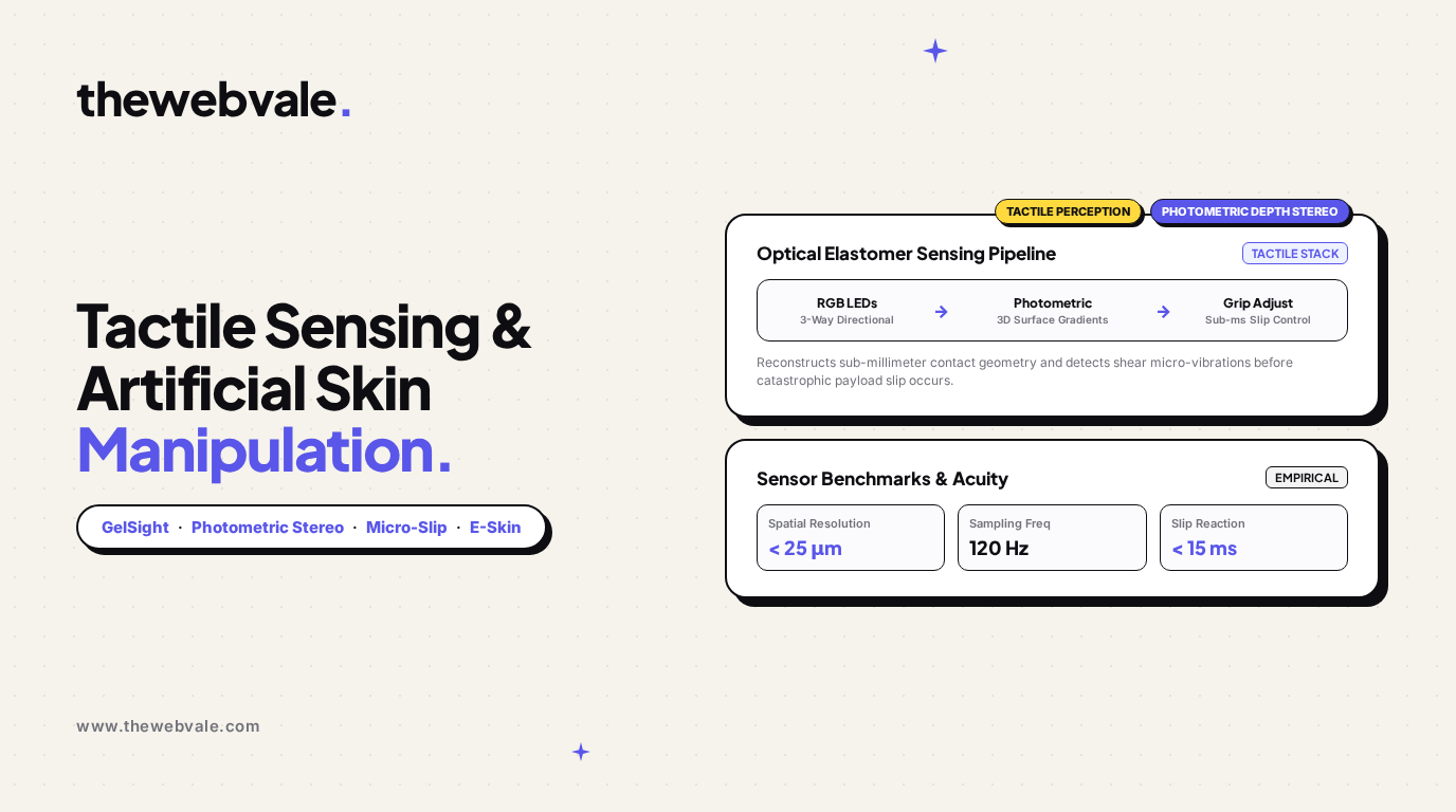
Optical-tactile sensors (such as MIT's GelSight, Meta's DIGIT, and GelSlim) solve the spatial resolution problem by converting tactile contact into an optical image. The sensor consists of a clear elastomeric dome coated on the outside with an opaque, semi-specular reflective paint (typically silicone mixed with microscopic aluminum powder), illuminated from three distinct angles by Red, Green, and Blue LEDs:
When an object (such as a threaded screw or fabric grain) presses into the gel membrane, it indents the surface. The internal micro-camera observes the indentation from behind. Because the membrane has uniform Lambertian reflectance and is illuminated from three known directional light source vectors [Lr, Lg, Lb], the surface gradient (p, q) at every single pixel (x, y) can be resolved in closed form:
Photometric Stereo Surface Normal Formulation:
I(x, y) = ρ · [ L ] · n(x, y)
Where I = [Ir, Ig, Ib]T is the observed RGB pixel intensity vector, L ∈ R3×3 is the calibrated illumination matrix, and n = [nx, ny, nz]T is the local unit surface normal vector:
n(x, y) = [ -p, -q, 1 ]T / √(1 + p2 + q2), where p = ∂z / ∂x and q = ∂z / ∂y
Once the gradient field (p, q) is extracted across all 300,000 pixels, the absolute 3D height profile z(x, y) is recovered by solving Poisson's equation via the Fast Fourier Transform (FFT):
Poisson Surface Reconstruction:
∇2 z(x, y) = (∂p / ∂x) + (∂q / ∂y)
This allows a robot to detect surface geometry at 25-micron spatial resolution—distinguishing the denomination of a coin or the weave density of denim purely through touch.
2. Comparison: Optical-Tactile vs. Electronic Skin (E-Skin)
Robotic hands employ different tactile modalities depending on the tradeoff between geometric spatial resolution, form-factor thickness, and mechanical durability:
| Tactile Technology | Spatial Resolution | Bandwidth (Hz) | Physical Thickness | Primary Advantage |
|---|---|---|---|---|
| Optical Elastomer (GelSight / DIGIT) | 20–50 μm (Camera pixels) | 60–120 Hz | 15–25 mm (Requires camera) | Sub-millimeter 3D contact topography |
| Piezoresistive E-Skin (Carbon Nanotubes) | 1.0–3.0 mm (Taxel grid) | 500–1,000 Hz | < 0.5 mm (Ultra-thin skin) | Wraps over multi-curved fingers & palm |
| Piezoelectric PVDF Dynamic Sensors | Discrete contact zones | > 2,000 Hz (Acoustic) | < 0.2 mm | Detects high-frequency micro-slip friction |
| Magnetic Hall-Effect Taxels (ReSkin) | 2.0–5.0 mm | 200–400 Hz | 2–4 mm | Extremely durable, low-cost replaceable skin |
3. The Mechanics of Incipient Micro-Slip
When a human grasps an object, the hand does not wait for the object to completely fall before tightening its grip. Instead, the nervous system detects incipient micro-slip: microscopic vibrations that occur within the outer annulus of the contact patch while the central contact core remains firmly stuck.
In robotics, this is captured by monitoring high-frequency spectral energy in the shear force signal:
Spectral Slip Index Formulation:
ξslip = [ ∫50 Hz..250 Hz |Sshear(f)|2 df ] / [ ∫0 Hz..50 Hz |Sshear(f)|2 df ]
When ξslip exceeds an empirical threshold τslip ≈ 1.8, the grasp controller automatically boosts normal clamping force ΔFN in under 15 milliseconds, terminating slip before any macroscopic movement occurs.
4. Production Implementation: Photometric Stereo 3D Contact Reconstruction
Below is a runnable Python production module providing a complete calibrated Photometric Stereo 3D reconstruction pipeline. It ingests simulated directional RGB tactile frames and solves Poisson's equation to reconstruct the 3D indentation depth map:
# Photometric Stereo 3D Tactile Surface Reconstruction
# GelSight / DIGIT Optical Elastomer Emulation

import numpy as np
from scipy.fft import fft2, ifft2
from typing import Tuple

class PhotometricTactileReconstructor:
    def __init__(self, height: int = 128, width: int = 128):
        self.H = height
        self.W = width

        # Calibrated 3x3 light source direction matrix L [Red, Green, Blue]
        # Angled at 120-degree radial increments with 45-degree elevation
        self.L = np.array([
            [ np.cos(0.0),            np.sin(0.0),            np.tan(np.radians(45.0))], # Red light
            [ np.cos(2.0*np.pi/3.0),   np.sin(2.0*np.pi/3.0),   np.tan(np.radians(45.0))], # Green light
            [ np.cos(4.0*np.pi/3.0),   np.sin(4.0*np.pi/3.0),   np.tan(np.radians(45.0))]  # Blue light
        ])
        # Normalize light vectors
        self.L = self.L / np.linalg.norm(self.L, axis=1, keepdims=True)
        self.L_inv = np.linalg.pinv(self.L)

    def reconstruct_normals_and_depth(self, rgb_image: np.ndarray) -> Tuple[np.ndarray, np.ndarray]:
        # rgb_image: Shape (H, W, 3) normalized in [0.0, 1.0]
        H, W, _ = rgb_image.shape
        flat_rgb = rgb_image.reshape(-1, 3).T # (3, H*W)

        # 1. Solve linear system: I = L * g  => g = L_inv * I
        g = self.L_inv @ flat_rgb # (3, H*W)

        # 2. Extract albedo and surface normals
        albedo = np.linalg.norm(g, axis=0) + 1e-6
        normals = g / albedo # Unit normals (3, H*W)
        normals = normals.T.reshape(H, W, 3)

        # Surface gradients: p = -n_x / n_z,  q = -n_y / n_z
        n_z = np.clip(normals[:, :, 2], 0.1, 1.0)
        p = -normals[:, :, 0] / n_z
        q = -normals[:, :, 1] / n_z

        # 3. Solve Poisson equation via Fourier Transform: div(p, q) = d2z/dx2 + d2z/dy2
        # Compute divergence of gradient field
        dp_dx = np.gradient(p, axis=1)
        dq_dy = np.gradient(q, axis=0)
        div = dp_dx + dq_dy

        # Frequency domain integration
        kx = 2.0 * np.pi * np.fft.fftfreq(W)
        ky = 2.0 * np.pi * np.fft.fftfreq(H)
        KX, KY = np.meshgrid(kx, ky)
        denom = -(KX**2 + KY**2)
        denom[0, 0] = 1.0 # Avoid division by zero at DC component

        div_fft = fft2(div)
        z_fft = div_fft / denom
        z_fft[0, 0] = 0.0 # Zero mean elevation

        depth_map = np.real(ifft2(z_fft))
        return normals, depth_map

# Demonstration with synthetic spherical indentation
if __name__ == "__main__":
    reconstructor = PhotometricTactileReconstructor(height=64, width=64)

    # Create synthetic spherical indentation (e.g. ball bearing pressed into gel)
    Y, X = np.ogrid[:64, :64]
    dist_sq = (X - 32)**2 + (Y - 32)**2
    radius = 16.0
    mask = dist_sq < radius**2

    true_depth = np.zeros((64, 64))
    true_depth[mask] = np.sqrt(radius**2 - dist_sq[mask]) * 0.1 # 1.6mm depth

    # Forward render synthetic RGB frame under calibrated 3-light setup
    true_p = np.gradient(true_depth, axis=1)
    true_q = np.gradient(true_depth, axis=0)
    true_normals = np.zeros((64, 64, 3))
    true_normals[:, :, 0] = -true_p
    true_normals[:, :, 1] = -true_q
    true_normals[:, :, 2] = 1.0
    true_normals /= np.linalg.norm(true_normals, axis=2, keepdims=True)

    flat_normals = true_normals.reshape(-1, 3).T
    synthetic_rgb = (reconstructor.L @ flat_normals).T.reshape(64, 64, 3)
    synthetic_rgb = np.clip(synthetic_rgb, 0.0, 1.0)

    # Run reconstruction
    est_normals, est_depth = reconstructor.reconstruct_normals_and_depth(synthetic_rgb)

    print("--- Optical-Tactile Photometric Stereo Reconstruction ---")
    print(f"Tactile Resolution: 64x64 Taxels ({reconstructor.H * reconstructor.W} points)")
    print(f"Max Indentation Depth Detected: {np.max(est_depth):.4f} mm")
    print(f"Normal Vector at Contact Apex (Center): [{est_normals[32, 32, 0]:+.3f}, {est_normals[32, 32, 1]:+.3f}, {est_normals[32, 32, 2]:+.3f}]")
5. Summary & Tactile Frontiers
Tactile sensing bridges the final chasm between machine vision and physical dexterity. By transforming soft elastomeric deformations into calibrated 3D depth maps and monitoring high-frequency shear micro-vibrations, artificial tactile skins endow robotic hands with the delicate compliance necessary to handle eggs, textiles, and surgical tools without crushing or dropping them. As sensor skins become thinner and integrated with onboard edge neural inference, physical robots will achieve true haptic fluency.