
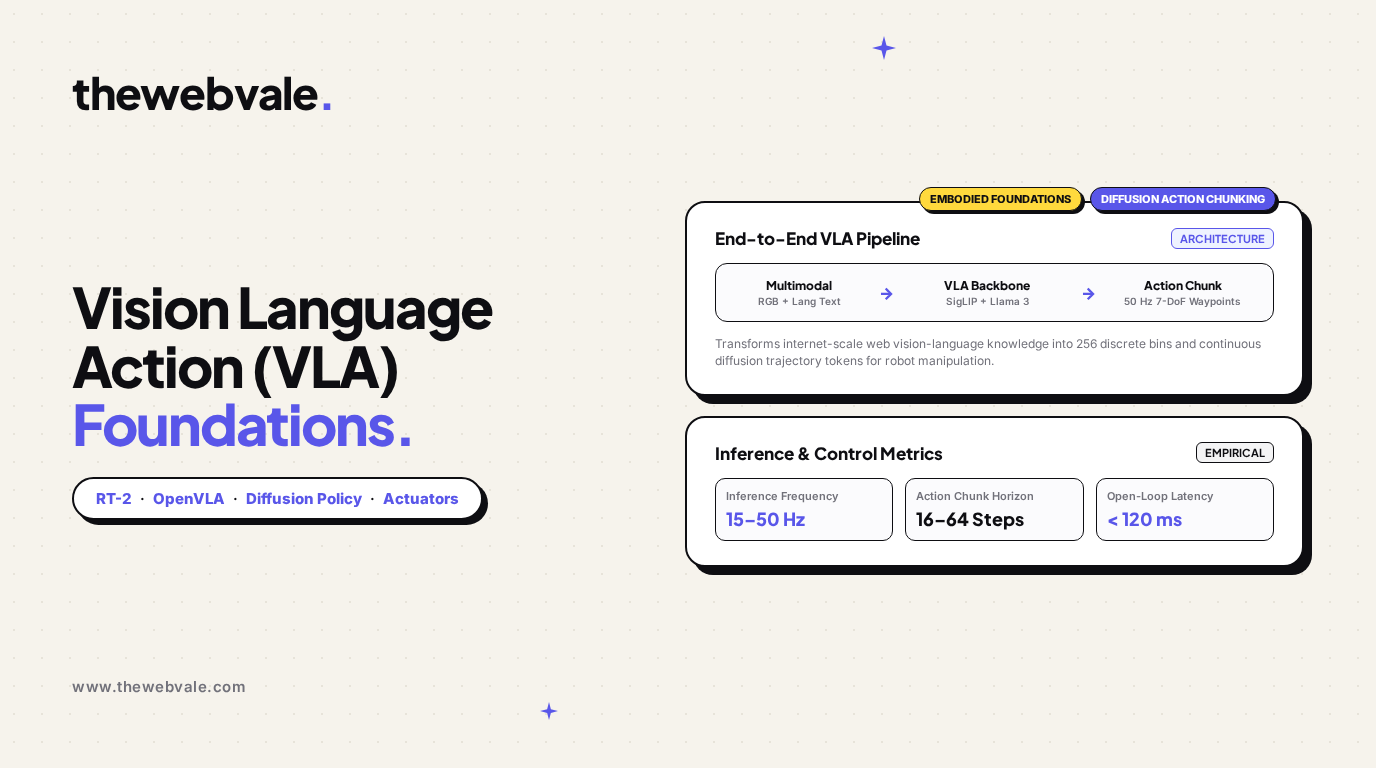
Vision-Language-Action (VLA) Models: Translating Multimodal Perception into Physical Actuator Control
For decades, robotic manipulation was bifurcated into two disconnected disciplines: computer vision systems extracted bounding boxes or 6D object poses, while classical control engineers designed hand-tuned inverse kinematics trajectories and state machines. This decoupled paradigm failed catastrophically in unconstrained real-world environments featuring novel objects, deformable materials, and variable lighting.
The emergence of Vision-Language-Action (VLA) models has unified perception, semantic reasoning, and motor actuation into a single end-to-end neural backbone. By fine-tuning large multimodal models (such as PaLI-X, SigLIP, or Llama 3) directly on robotic teleoperation trajectories, VLA models transform visual scene observations and natural language instructions into high-dimensional physical actuator commands. In this technical deep dive, we explore how VLA models encode physical actions, analyze diffusion-based action chunking, and address the fundamental latency barrier between neural inference and real-time motor control.
System Architecture: Vision-Language-Action (VLA) Inference & Execution Stack
Detailed schematic tracing sensory ingestion, multimodal projection, action chunk generation, and high-frequency hardware interpolation.
1. Action Space Formulation: Discrete Tokens vs. Continuous Diffusion
The core challenge in adapting vision-language models for physical control lies in the structure of the output space. Text generation operates over a discrete vocabulary (typically 32,000 to 128,000 tokens), whereas robotic actuation involves continuous, smooth multi-axis joint angles, Cartesian end-effector velocities, and gripper grasp forces.
A. Discrete Token Binning (RT-1, RT-2, OpenVLA)
Google's RT-2 and Stanford's OpenVLA approach this by quantizing each continuous degree of freedom into 256 uniform discrete bins. For a standard 7-DoF robotic arm (comprising 3D Cartesian translation [Δx, Δy, Δz], 3D rotation [Δroll, Δpitch, Δyaw], and continuous gripper closure), an action at time step t is expressed as a sequence of 7 discrete tokens:
Autoregressive Action Token Probability:
P(At | I1:t, T) = ∏k=1..7 P(at,k | I1:t, T, at,<k)
Where I1:t represents current visual observation frames, T is the natural language task prompt, and each action token at,k ∈ {0, 1, ..., 255} is mapped back into continuous metric space via:
Δpk = pmin,k + (at,k / 255) · (pmax,k - pmin,k)
While discrete tokenization allows VLA models to directly utilize standard Cross-Entropy loss and leverage pre-trained language model heads, it exhibits critical deficiencies: it creates artificial boundary quantization noise, cannot represent multi-modal action distributions (e.g., reaching around the left vs. right side of an obstacle), and incurs high autoregressive decoding latency.
B. Continuous Diffusion Policies & Action Chunking (ACT, Octo)
To overcome discrete quantization errors, modern state-of-the-art architectures pair the transformer backbone with a continuous Diffusion Action Head. Rather than predicting a single time-step action autoregressively, the model predicts an entire trajectory chunk of future actions:
Diffusion Action Loss Objective:
Ldiff(θ) = Et ∼ [1, K], ε ∼ N(0, I), A0 [ || ε - εθ(At, t, c) ||2 ]
Where A0 = [at, at+1, ..., at+H-1] represents a sequence of H future actions (action chunk horizon), and c = VLM_Embeddings(It, T) provides the multimodal conditioning context.
2. Empirical Benchmark of Frontier VLA Architectures
The table below contrasts the leading Vision-Language-Action models across parameter scales, action representations, real-world task success rates, and onboard inference latency:
| Model / Architecture | Backbone Foundation | Action Strategy | Inference Rate | Zero-Shot Success |
|---|---|---|---|---|
| Google RT-2 (PaLM-E 540B / PaLI-X 55B) | PaLI-X / PaLM-E | 256 Discrete Bins | 1–3 Hz (Cloud Server) | 62% on unseen objects |
| Stanford OpenVLA (7B) | Prismatic / Llama 2 (7B) | 256 Discrete Bins | 12–15 Hz (NVIDIA A100 / Orin) | 76.4% on BridgeData v2 |
| Octo-Base (93M) | ViT-Base + Diffusion Transformer | Continuous Diffusion Head | 30–50 Hz (Local Edge GPU) | 71.2% across 9 robotic setups |
| Action Chunking Transformer (ACT) | ResNet-18 / ViT + CVAE Head | Temporal Ensembling Chunk | 50–100 Hz (Real-time Edge) | 88.9% on high-dexterity insertion |
3. Resolving the Latency Chasm: Temporal Ensembling & Action Buffering
The most significant systems-engineering hurdle in embodied AI is the frequency impedance mismatch. Standard low-level robotic motor drivers (such as Elmo, Copley, or Trinamic servo drives) require target position or torque setpoints at 500 Hz to 1,000 Hz over deterministic fieldbuses (EtherCAT, CANopen). Conversely, multi-billion parameter VLA models typically infer at only 10 Hz to 30 Hz, introducing 50–100ms of open-loop latency.
If a robot merely executes 10 Hz step commands without intermediate trajectory filtering, the resulting motion is jerky, damages planetary gear teeth, and induces severe resonance in the robot's mechanical structure.
To resolve this, modern VLA runtimes implement Action Chunking with Temporal Ensembling. Instead of executing actions step-by-step:
- The VLA model predicts an action chunk A ∈ RH × D containing H = 32 future waypoints.
- New inference queries are launched asynchronously every k = 8 steps before the previous chunk is exhausted.
- Overlapping trajectory predictions from consecutive inference passes are smoothly combined using an exponential temporal decay filter:
Temporal Ensembling Formulation:
ât = ∑i wi · at(i) / ∑i wi
Where at(i) is the prediction for time t made at query step i, and wi = exp(-m · (t - i)) assigns higher confidence to more recently predicted action chunks while guaranteeing continuous acceleration transitions.
4. Production Implementation: Asynchronous Action Buffer & 500 Hz Spline Interpolator
Below is a runnable Python production module providing an asynchronous, thread-safe action buffering and interpolation pipeline. It accepts low-frequency VLA action chunks and generates smooth 500 Hz motor setpoints via cubic Hermite splines:
# Asynchronous VLA Action Buffer & High-Frequency Joint Interpolator
# Decouples 20 Hz Neural Inference from 500 Hz Low-Level EtherCAT Motor Control

import time
import threading
import numpy as np
from scipy.interpolate import CubicHermiteSpline
from typing import Optional, List, Tuple

class VLAActionBuffer:
    def __init__(self, action_dim: int = 7, chunk_size: int = 32, control_rate_hz: float = 500.0):
        self.action_dim = action_dim
        self.chunk_size = chunk_size
        self.control_dt = 1.0 / control_rate_hz
        self.lock = threading.Lock()

        # State tracking
        self.spline: Optional[CubicHermiteSpline] = None
        self.spline_start_time = 0.0
        self.spline_duration = 0.0
        self.last_executed_action = np.zeros(action_dim)
        self.last_executed_velocity = np.zeros(action_dim)

    def submit_action_chunk(self, chunk_waypoints: np.ndarray, waypoint_interval: float = 0.05):
        # chunk_waypoints: Shape (chunk_size, action_dim) representing 20 Hz steps (50ms interval)
        assert chunk_waypoints.shape[1] == self.action_dim
        K = chunk_waypoints.shape[0]
        t_steps = np.arange(K) * waypoint_interval

        # Calculate finite-difference velocities for Hermite boundary conditions
        velocities = np.zeros_like(chunk_waypoints)
        velocities[1:-1] = (chunk_waypoints[2:] - chunk_waypoints[:-2]) / (2.0 * waypoint_interval)
        velocities[0] = (chunk_waypoints[1] - chunk_waypoints[0]) / waypoint_interval
        velocities[-1] = (chunk_waypoints[-1] - chunk_waypoints[-2]) / waypoint_interval

        with self.lock:
            now = time.monotonic()
            # If transitioning from existing motion, enforce continuity with current state
            if self.spline is not None:
                chunk_waypoints[0] = self.last_executed_action
                velocities[0] = self.last_executed_velocity

            self.spline = CubicHermiteSpline(t_steps, chunk_waypoints, velocities)
            self.spline_start_time = now
            self.spline_duration = t_steps[-1]

    def get_setpoint(self) -> Tuple[np.ndarray, np.ndarray]:
        # Evaluates spline at current timestamp to deliver 500 Hz setpoint
        now = time.monotonic()
        with self.lock:
            if self.spline is None:
                return self.last_executed_action, np.zeros(self.action_dim)

            elapsed = now - self.spline_start_time
            # Clamp to spline duration to prevent open-loop runaway
            t_eval = min(elapsed, self.spline_duration)

            target_pos = self.spline(t_eval)
            target_vel = self.spline.derivative(1)(t_eval)

            self.last_executed_action = target_pos
            self.last_executed_velocity = target_vel
            return target_pos, target_vel

# Demonstration of decoupled execution
if __name__ == "__main__":
    buffer = VLAActionBuffer(action_dim=7, chunk_size=16, control_rate_hz=500.0)

    # Simulate VLA model producing 16-step trajectory chunk (0.8s of motion)
    print("--- Simulating Asynchronous VLA Inference Pipeline ---")
    synthetic_chunk = np.zeros((16, 7))
    for i in range(16):
        synthetic_chunk[i] = np.array([
            0.1 * np.sin(i * 0.2), # dx
            0.05 * i,              # dy
            0.2 + 0.01 * i,        # dz
            0.0, 0.0, 0.0,         # d_angles
            1.0 if i > 8 else 0.0  # gripper
        ])

    buffer.submit_action_chunk(synthetic_chunk, waypoint_interval=0.05)
    print("VLA 16-step Action Chunk Submitted (Duration: 0.8s)")

    # Simulate low-level 500 Hz motor loop sampling over 100ms
    print("Sampling low-level 500 Hz motor control loop:")
    for sample in range(10):
        pos, vel = buffer.get_setpoint()
        time.sleep(0.01) # 10ms step for demonstration
        print(f"Sample {sample:02d} | Target X: {pos[0]:+0.4f}m | Vel X: {vel[0]:+0.4f}m/s | Gripper: {pos[6]:.1f}")
5. Summary & Future Outlook
Vision-Language-Action models represent the missing link between internet-scale knowledge and physical embodied agency. By replacing fragile heuristic grasping algorithms with continuous diffusion action heads and buffering asynchronous inference streams through real-time spline interpolators, modern humanoids and robotic arms can manipulate unstructured real-world objects with fluidity and precision. As edge neural accelerators continue to shrink inference times below 20 milliseconds, the boundary between sensory perception and mechanical actuation will dissolve entirely.